The mouse cortico-basal ganglia-thalamic network
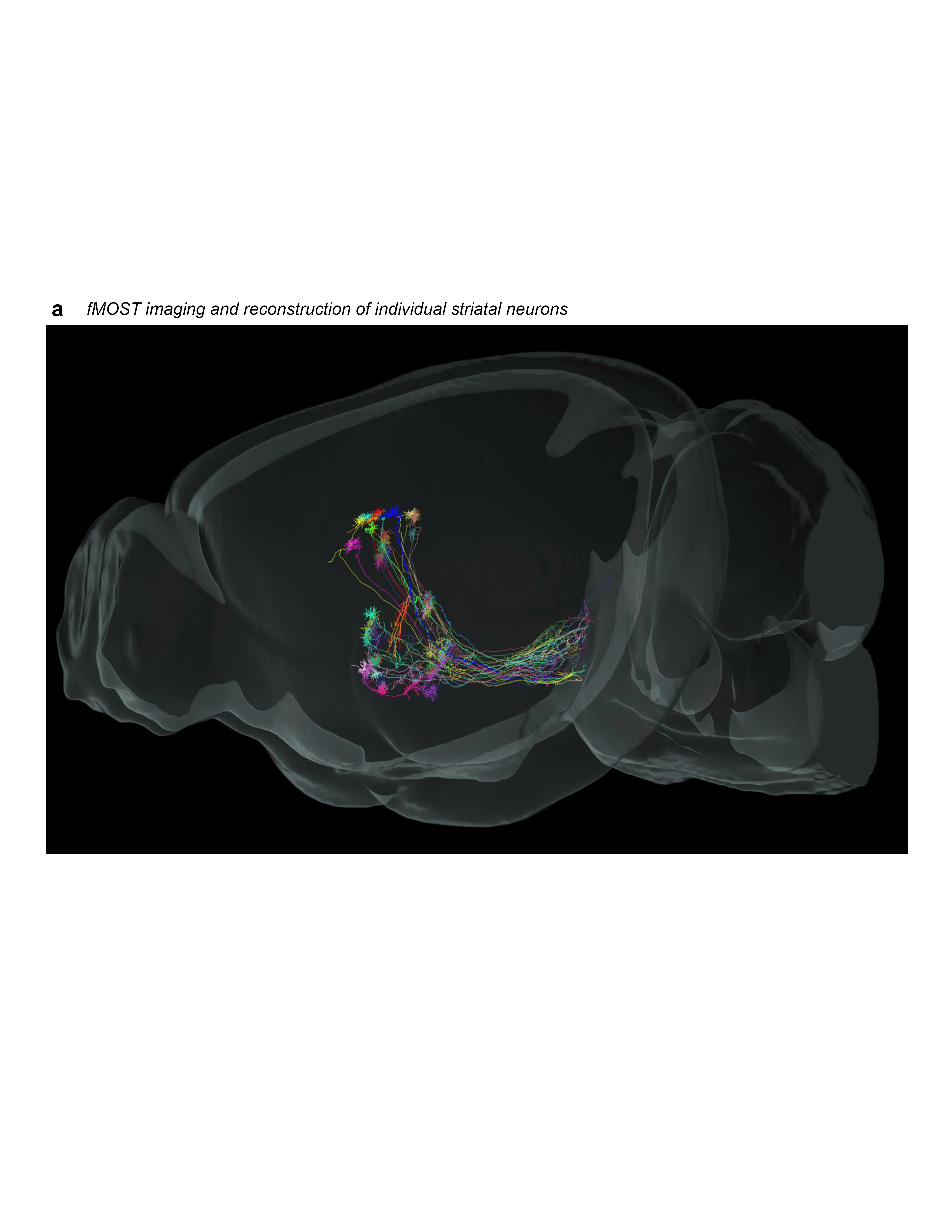
The cortico-basal ganglia-thalamo-cortical loop is one of the fundamental network motifs in the brain. Revealing its structural and functional organization is critical to understanding cognition, sensorimotor behavior, and the natural history of many neurological and neuropsychiatric disorders. Classically, this network is conceptualized to contain three information channels: motor, limbic, and associative. Yet this three-channel view cannot explain the myriad functions of the basal ganglia. We previously subdivided the dorsal striatum into 29 functional domains based on the topography of inputs from the entire cortex (Hintiryan et al. 2016). Here, we map the multi-synaptic output pathways of these striatal domains through the globus pallidus external part (GPe), substantia nigra reticular part (SNr), thalamic nuclei, and cortex. Accordingly, we identify 14 SNr and 36 GPe domains and a direct cortico-SNr projection. The striatonigral direct pathway displays a greater convergence of striatal inputs than the more parallel striatopallidal indirect pathway, although direct and indirect pathways originating from the same striatal domain ultimately converge onto the same postsynaptic SNr neurons. Following the SNr outputs, we delineate 6 domains in the parafascicular and ventromedial thalamic nuclei. Subsequently, we identify 6 parallel cortico-basal ganglia-thalamic subnetworks that sequentially transduce specific subsets of cortical information through every elemental node of the cortico-basal ganglia-thalamic loop. Thalamic domains relay this output back to the originating corticostriatal neurons of each subnetwork in a bona fide closed loop.
Cortex (Video) ![]() | SNr reconstructions (SWC)
| SNr reconstructions (SWC) ![]()
Raw Data (CSV)
|
|
|
|
|||
|
|
|
|
|||
|
|
|
|
|||
|
|
|
|

Tables
|
|
|
|
Figures
|
Figure 1.jpg
|
 |
|
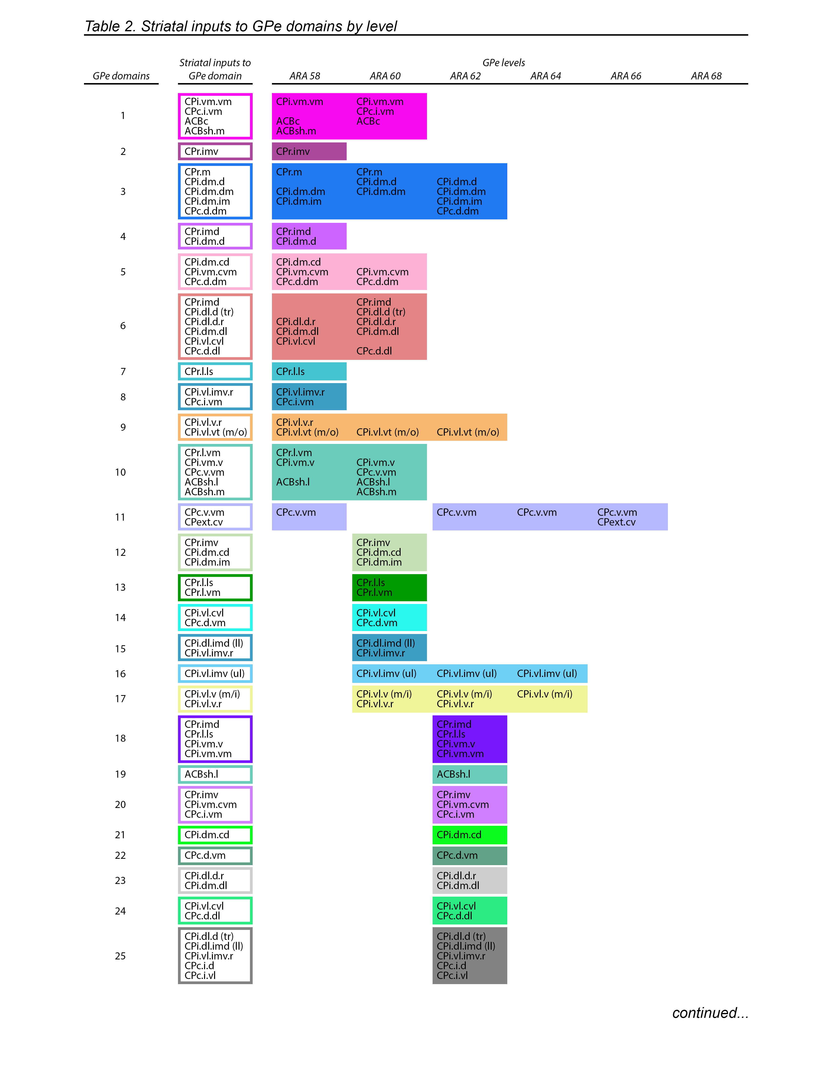
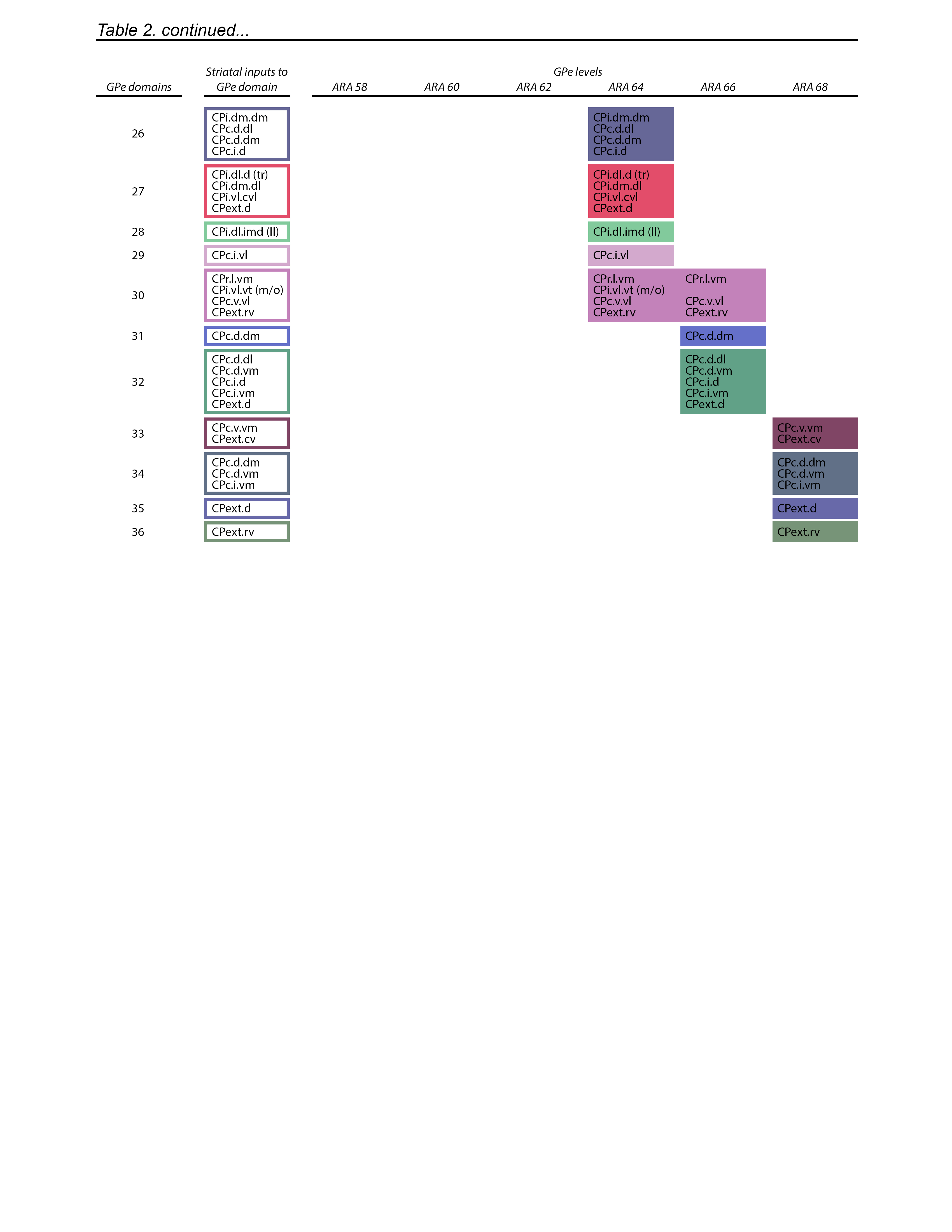
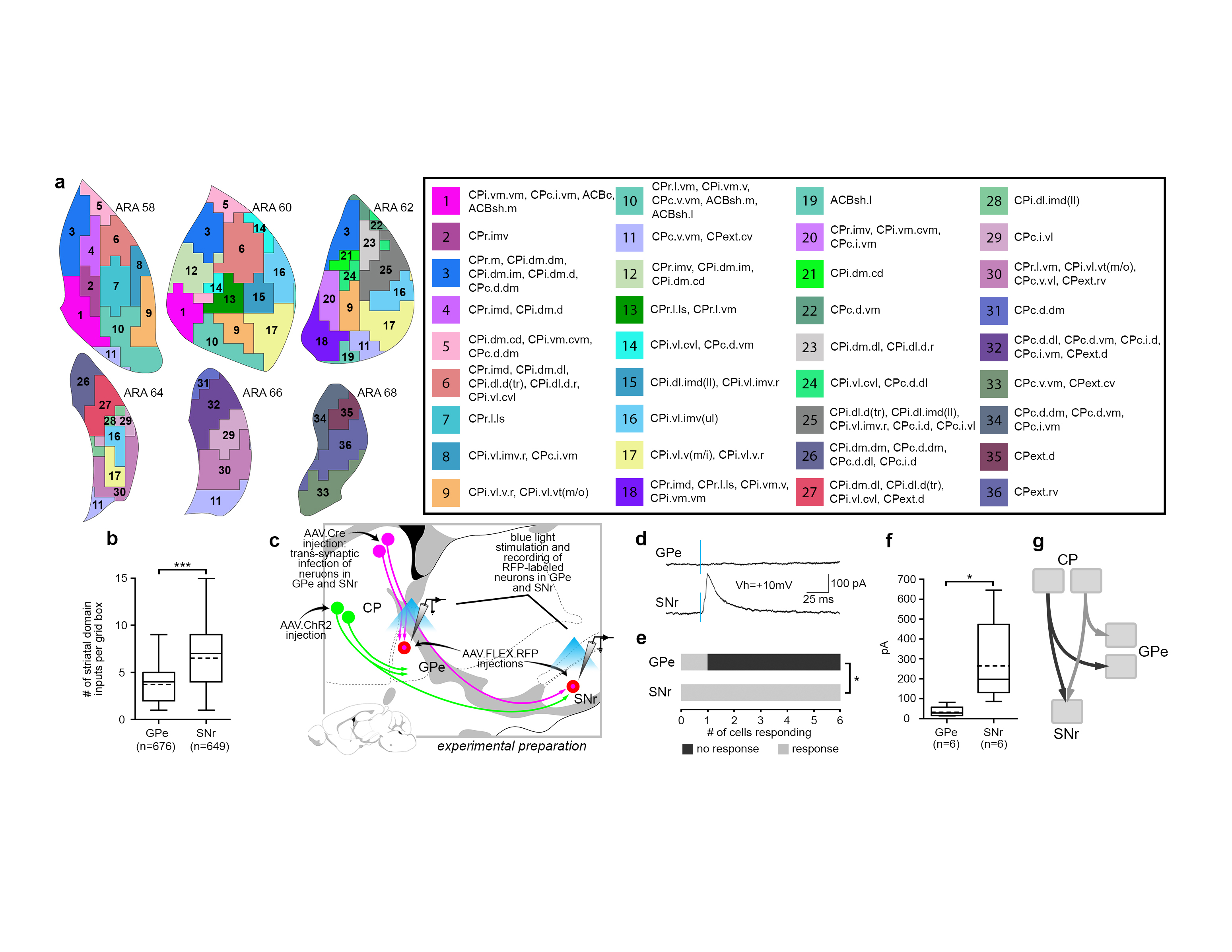
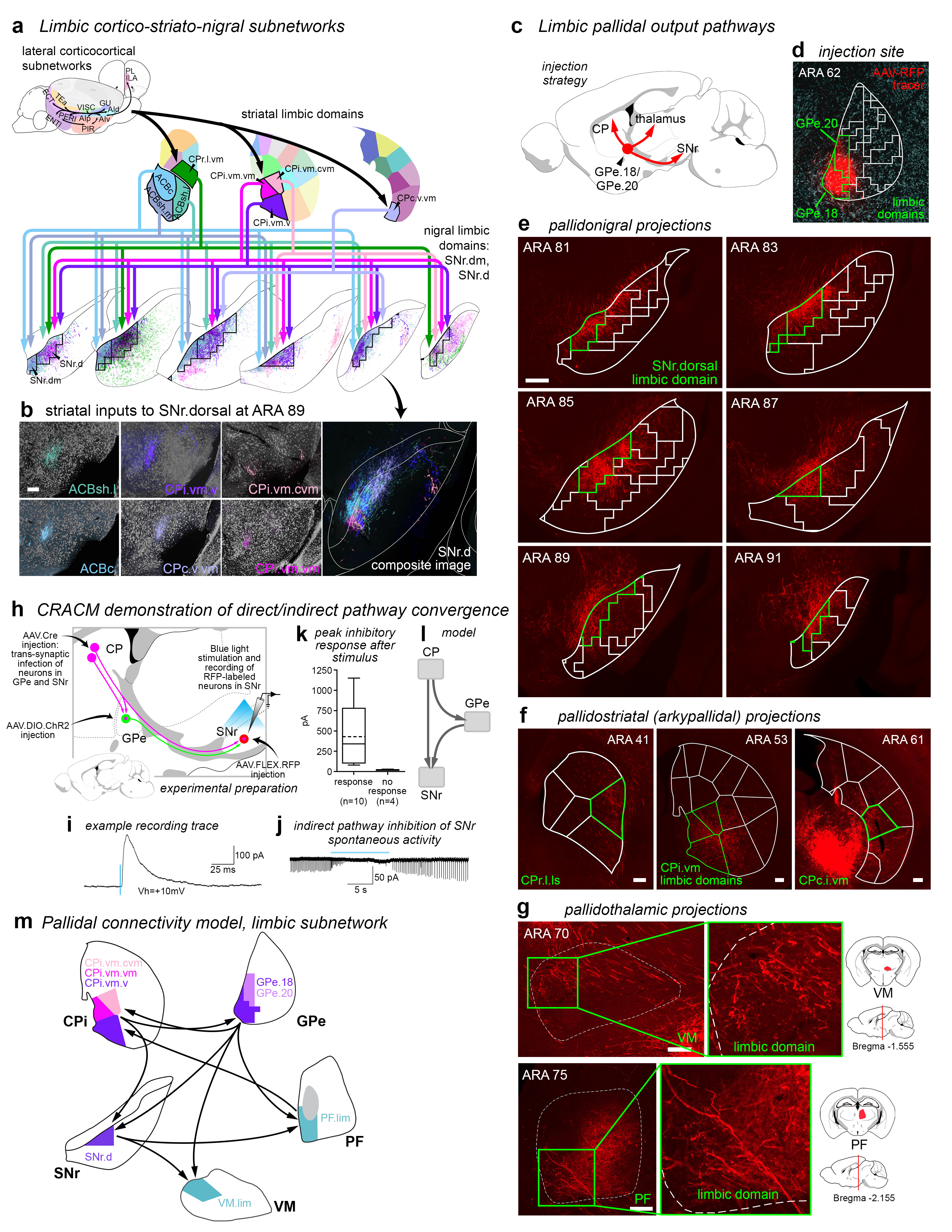
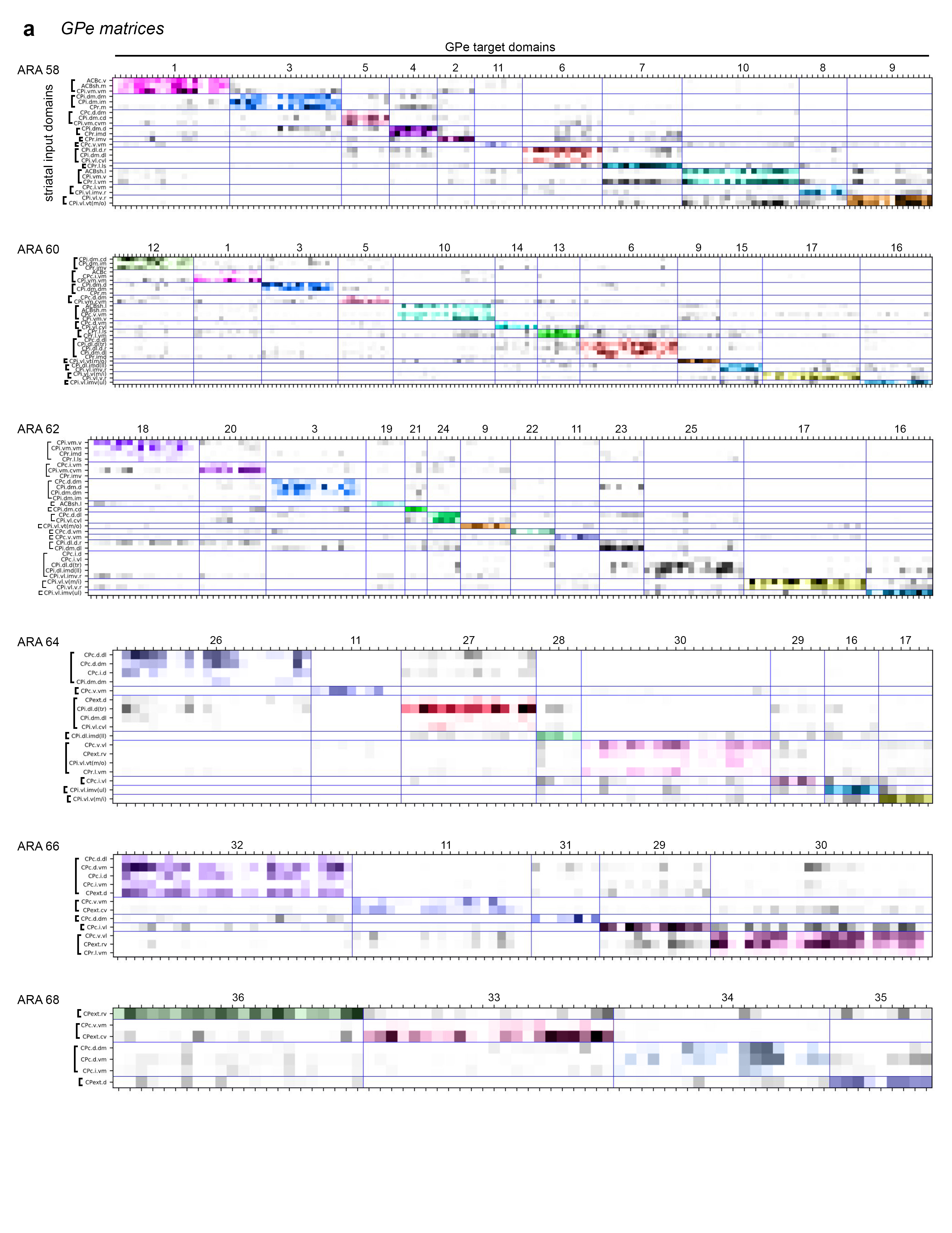
Figure 2.jpg Figure 2. Indirect pathway defines GPe domain structure and differs from direct pathway. a, Striatal axonal inputs (see Extended Data Fig. 11) define GPe domains. Legend for GPe domain map (right) lists striatal inputs. b, Analysis of grid box data reveals that the mean number of striatal domains providing inputs to each grid box differs significantly between GPe and SNr, indicating greater convergence in the direct pathway (mean±sd, GPe: 3.75±1.79, SNr: 6.49±2.97, P<.0001, 2-tailed t test, t=20.26, df=1057). Total numbers of grid boxes in GPe (n=676) and SNr (n=649) are similar, meaning their gross volumes are similar. c, Schematic of experimental strategy for electrophysiological test of parallelism in indirect pathway and convergence in direct pathway. d, Example recording traces from RFP-tagged neurons in GPe and SNr. e, Number of neurons responding to stimulus was significantly different between GPe (n=6) and SNr (n=6; P=.0152, Fisher’s exact test, 3 mice). f, Peak amplitude of current after stimulation was significantly different between GPe and SNr neurons (mean±sd, GPe: 33.67±24.74 pA; SNr: 267.5±197.6 pA; P=.0348, 2-tailed t test, t=2.876, df=5). g, Simplified schematic of the direct and indirect pathways. For box plots, boxes demarcate first/third quartiles, whiskers show min/max, solid line is median, dashed line is mean. |
 |
|
Figure 3.jpg
|
 |
|
Figure 4.jpg
|
 |
|
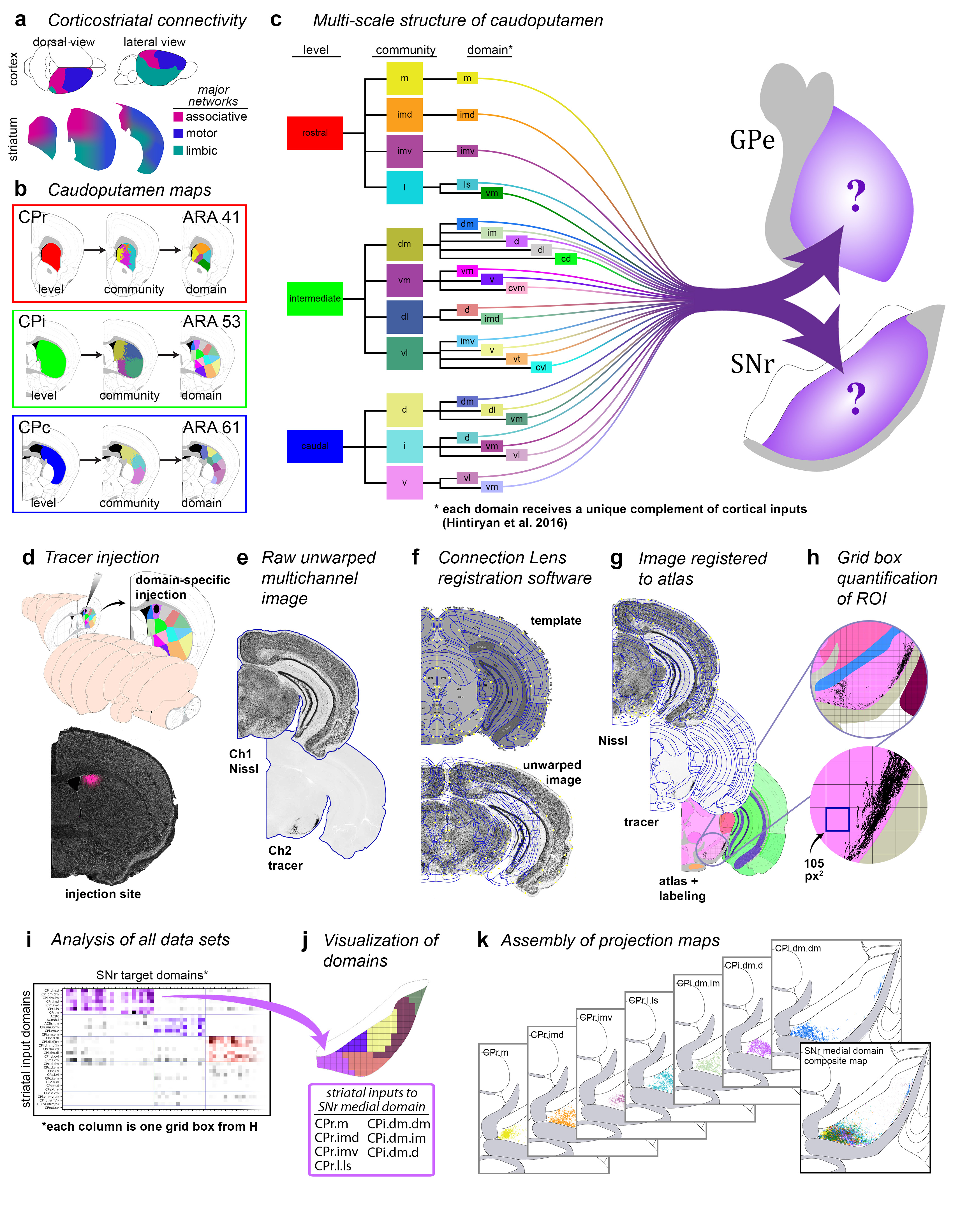
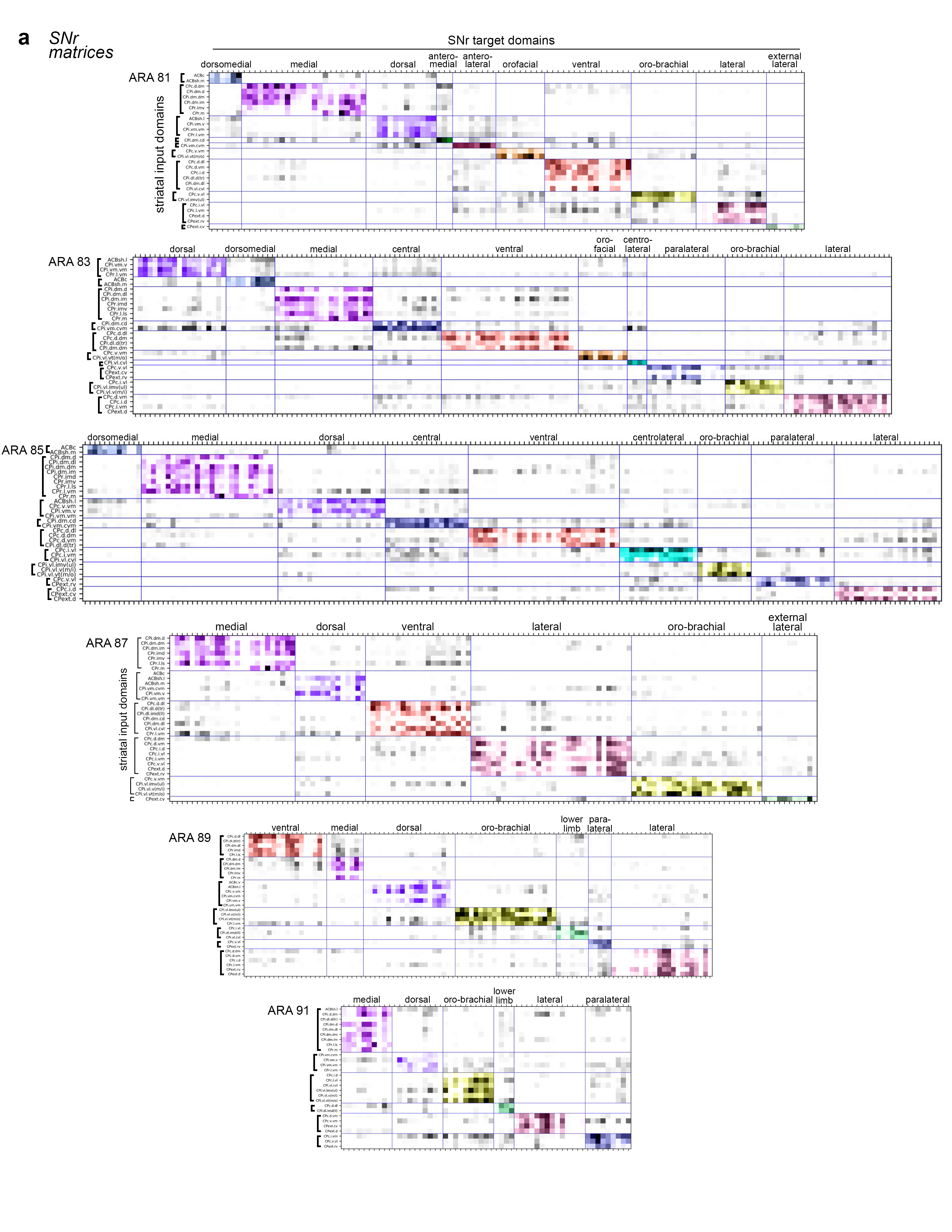
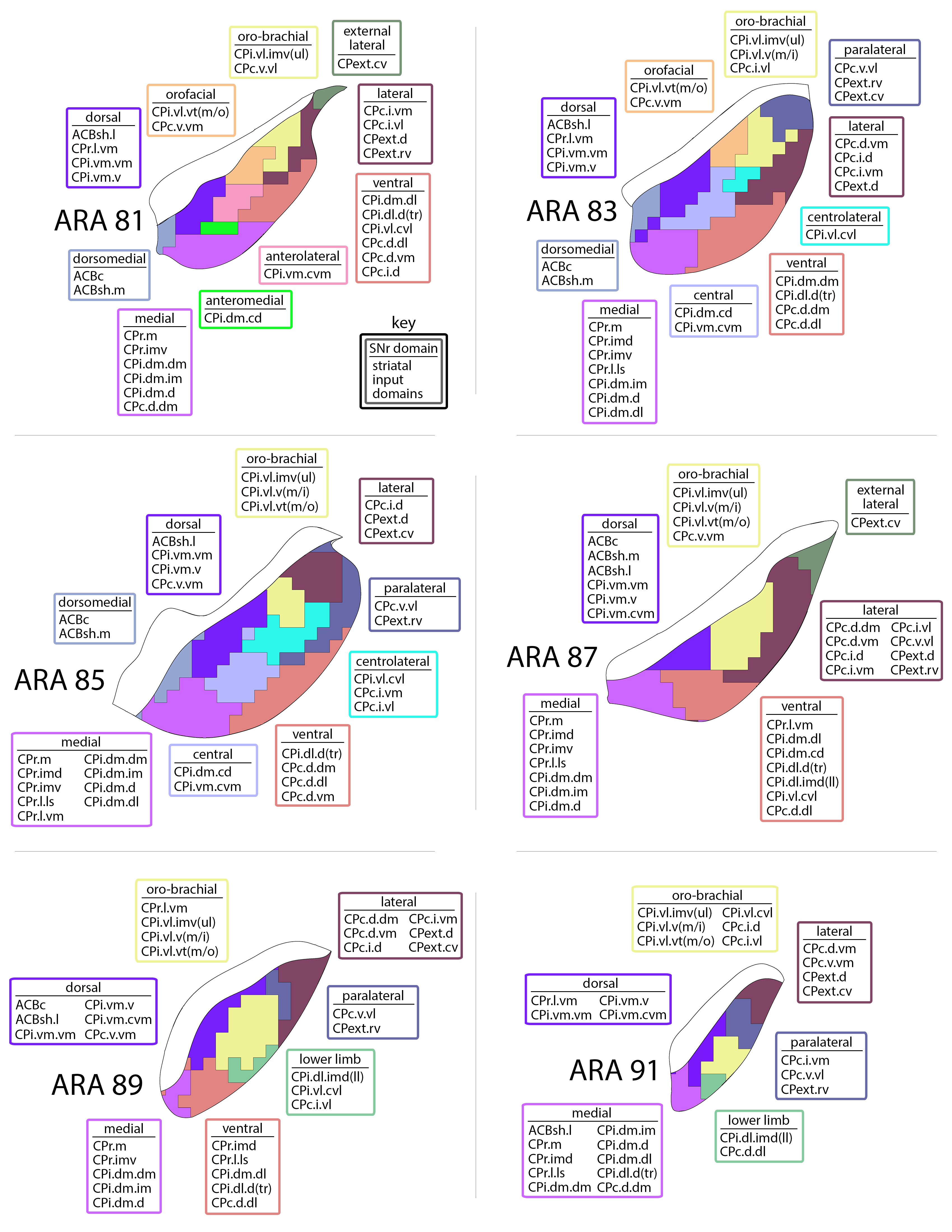
Extended Data Figure 1.jpg Extended Data Figure 1. Rationale and workflow for the striatal output analysis. a, General topography of the 3 classic corticostriatal pathways: motor, limbic, and associative. b, Map of the multi-scale subdivisions (level>community>domain) of the caudoputamen at rostral (CPr), intermediate (CPi), and caudal (CPc) levels. c, Dendrogram of the multi-scale, hierarchical structure of the CP, depicting how each level is composed of smaller communities and even smaller domains, each with a unique set of cortical inputs. The precise topography of the striatal output pathway is unknown. The CP caudal extreme and nucleus accumbens domains are not depicted here but were analyzed. The data production workflow starts with d, discrete injection of anterograde tracer into one of the striatal domains. Tissue sections are e, imaged and imported into f, Connection Lens where fiducial points in the nissl channel are matched to the atlas template. g, Images are deformably warped and the tracer channel is segmented into a binary threshold image. h, The software subdivides all brain regions into a square grid space and quantifies the pixels of axon labeling in each grid box. i, The quantified axonal terminals from all injections to all grid boxes at each nucleus-level is visually summarized in a matrix (darker shading indicates denser termination; colors correspond to particular SNr domains). Statistical analysis reveals the subnetworks, groups of striatal domains that project to a common set of grid boxes. Those grid boxes in the SNr maps are then j, colored to visualize the new input-defined pallidal or nigral domain. k, Composite projection maps of the colored axonal terminals illustrate the striatofugal terminal pattern, with axonal color matching the source domain from the striatal domain map. |
 |
|
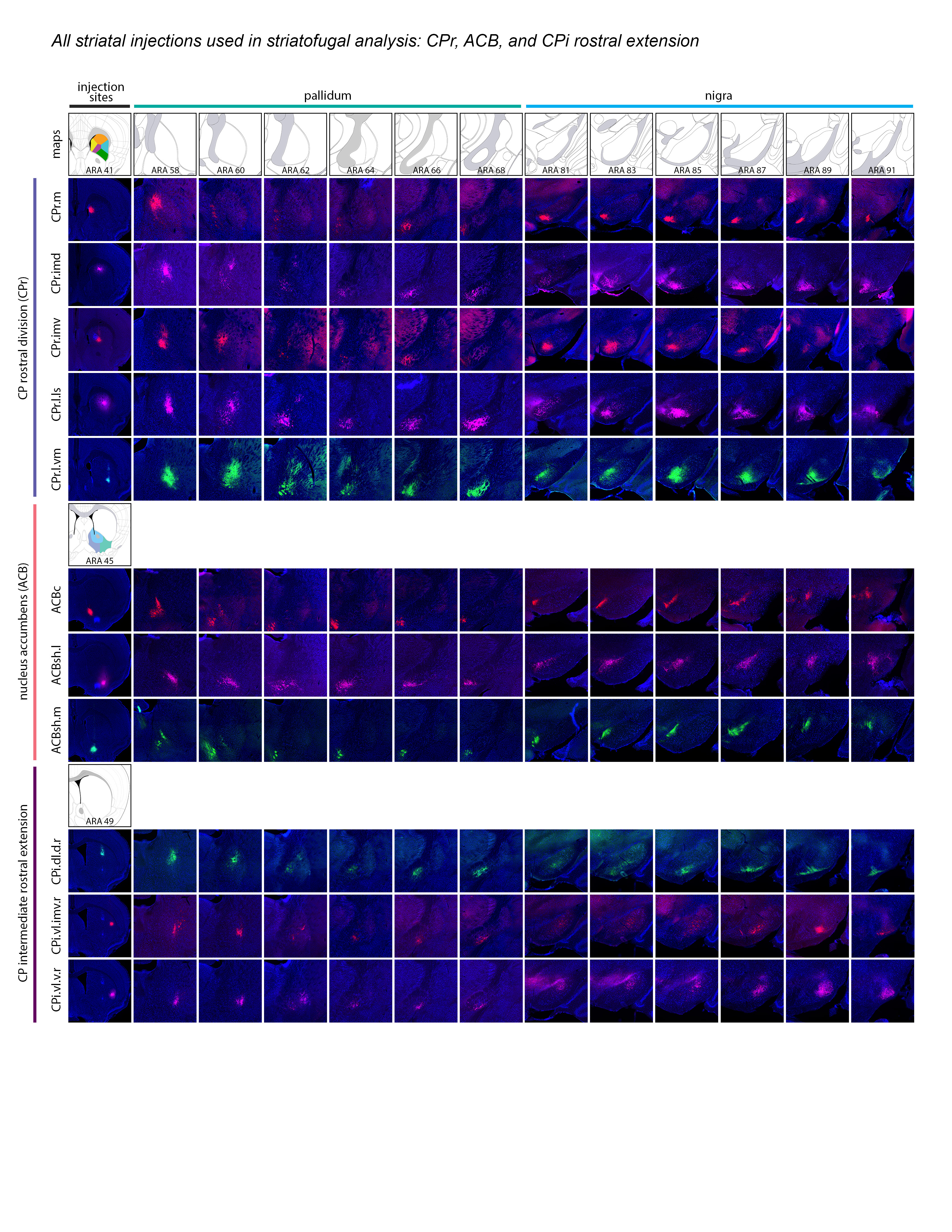
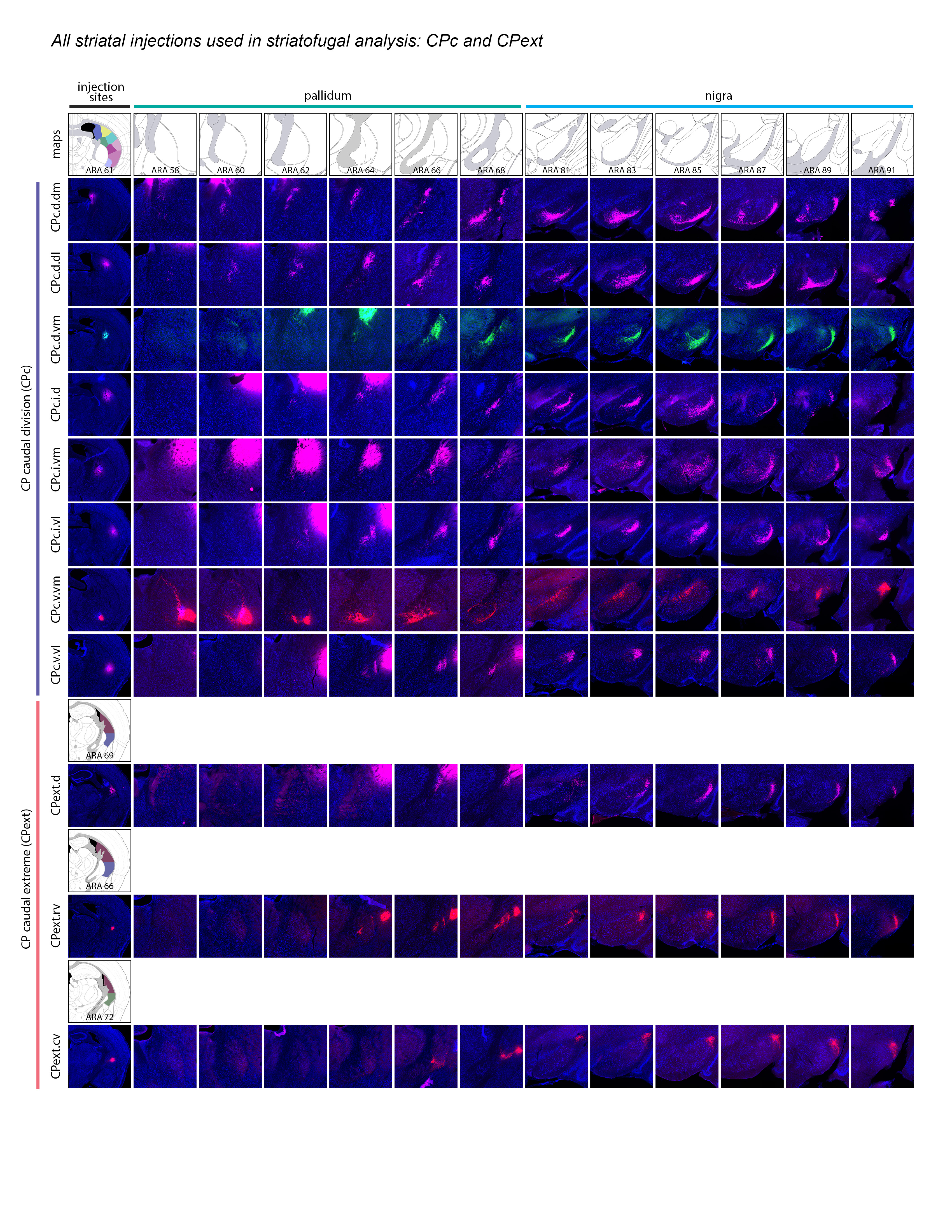
Extended Data Figure 2 1of3.jpg Extended Data Figure 2. All 36 striatal injections used in the striatal output analysis. The injection sites and raw axonal labeling at each representative level of the pallidum and nigra are shown. Rostral CP, nucleus accumbens, and intermediate CP rostral extension are shown on the first page; intermediate CP is shown on the second page; and caudal CP and caudal extreme are shown on the third page. These images were analyzed to determine the 14 nigral and 36 pallidal domains. The entire striatal output dataset was subjected to computational analysis with the Louvain algorithm, revealing the domain structure at each representative level of the GPe and SNr (every other level of each structure). The CP intermediate rostral extension injections were included in the GPe analysis but not the SNr analysis, since those injections labeled unique areas in GPe but had labeling highly similar to their CPi-level counterparts (i.e., the CPi.dl.imd, CPi.vl.imv, and CPi.vl.v). All images are coronal, medial is left.
|
 |
| Extended Data Figure 2 2of3.jpg | 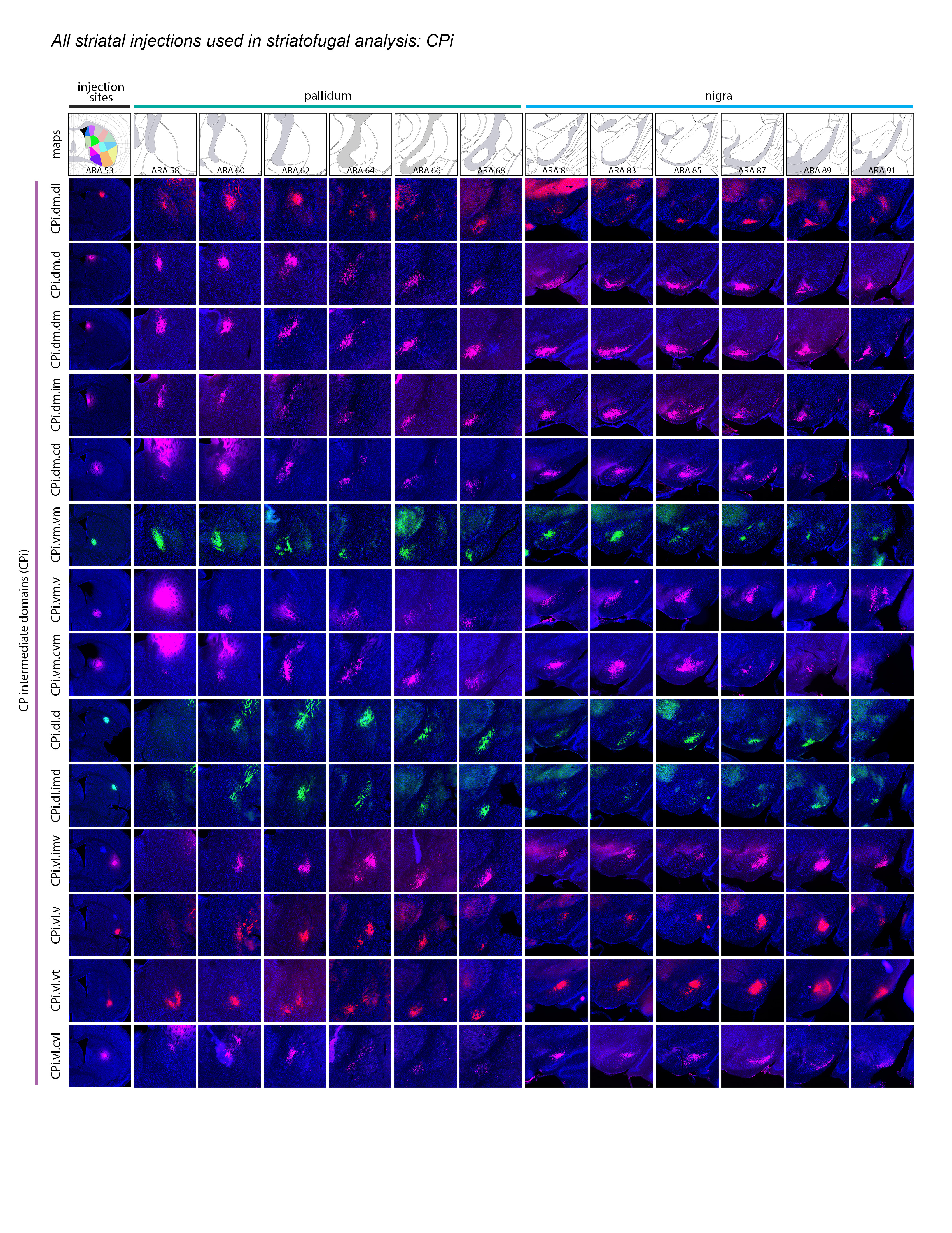 |
|
Extended Data Figure 2 3of3.jpg |
 |
|
Extended Data Figure 3.jpg
|
 |
|
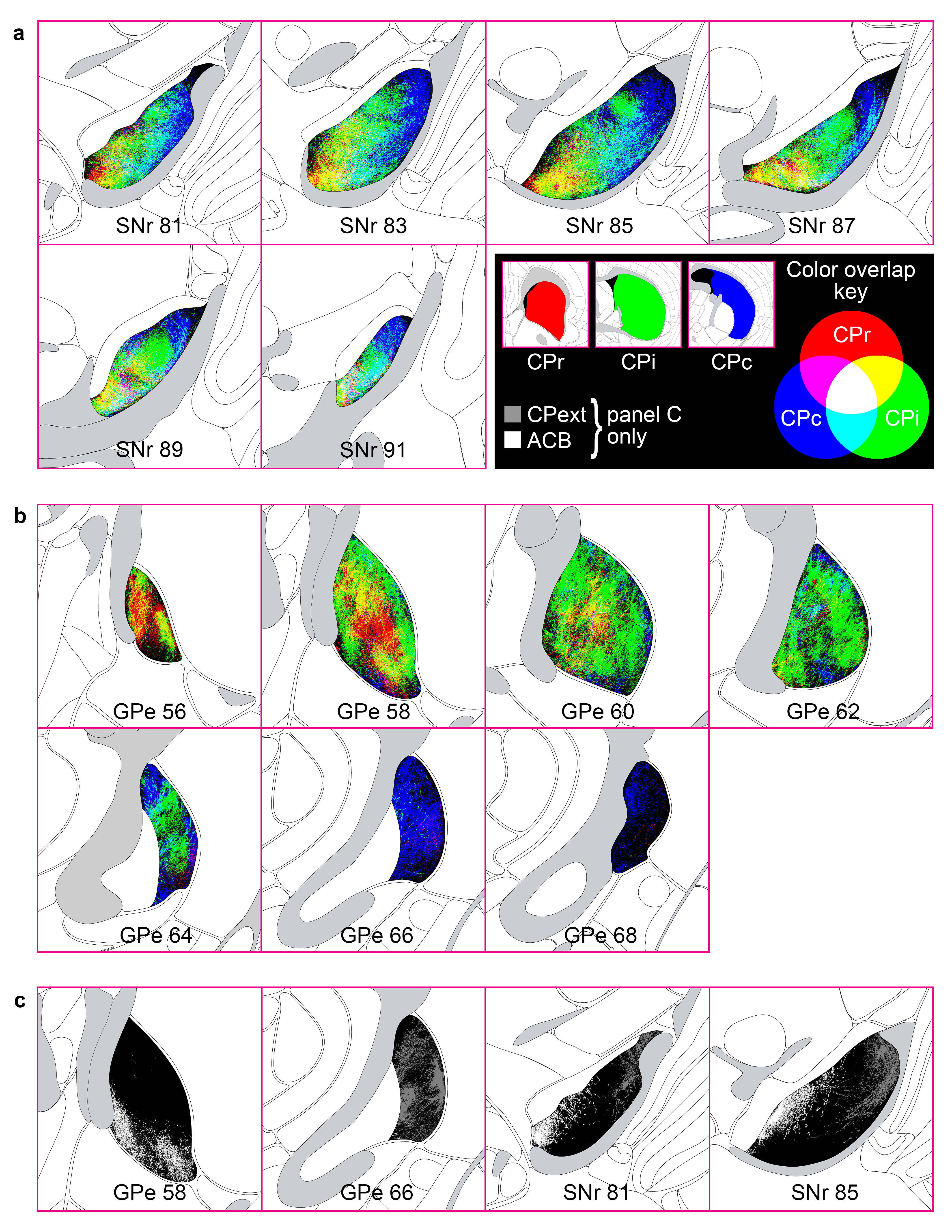
Extended Data Figure 4.jpg Extended Data Figure 4. Striatal level topographic trends, blended-color style emphasizing convergence. Similar to the striatal level maps presented in Extended Data Figs. 3a and 11c, the maps here present the striatal level termination patterns in red, green, and blue for CPr, CPi, and CPc, respectively, but when axons from different divisions overlap, the pixel color is a blended RGB value of the constituent axons (see Color overlap key). The maps in Extended Data Figs. 3a and 11c were made with opaque layers (CPr>CPi>CPc, top to bottom) such that pixels of axon in the upper layers occlude any other axons in lower layers in the same pixel; those maps were meant to emphasize the differences in level-scale terminal patterns, whereas the maps in this figure emphasize the areas of overlap within a SNr and b GPe. The terminations of the ACB and CPext (also known as the tail of the caudate) are shown in grayscale in c. |
 |
|
Extended Data Figure 5.jpg
|
 |
|
Extended Data Figure 6.jpg
|
 |
|
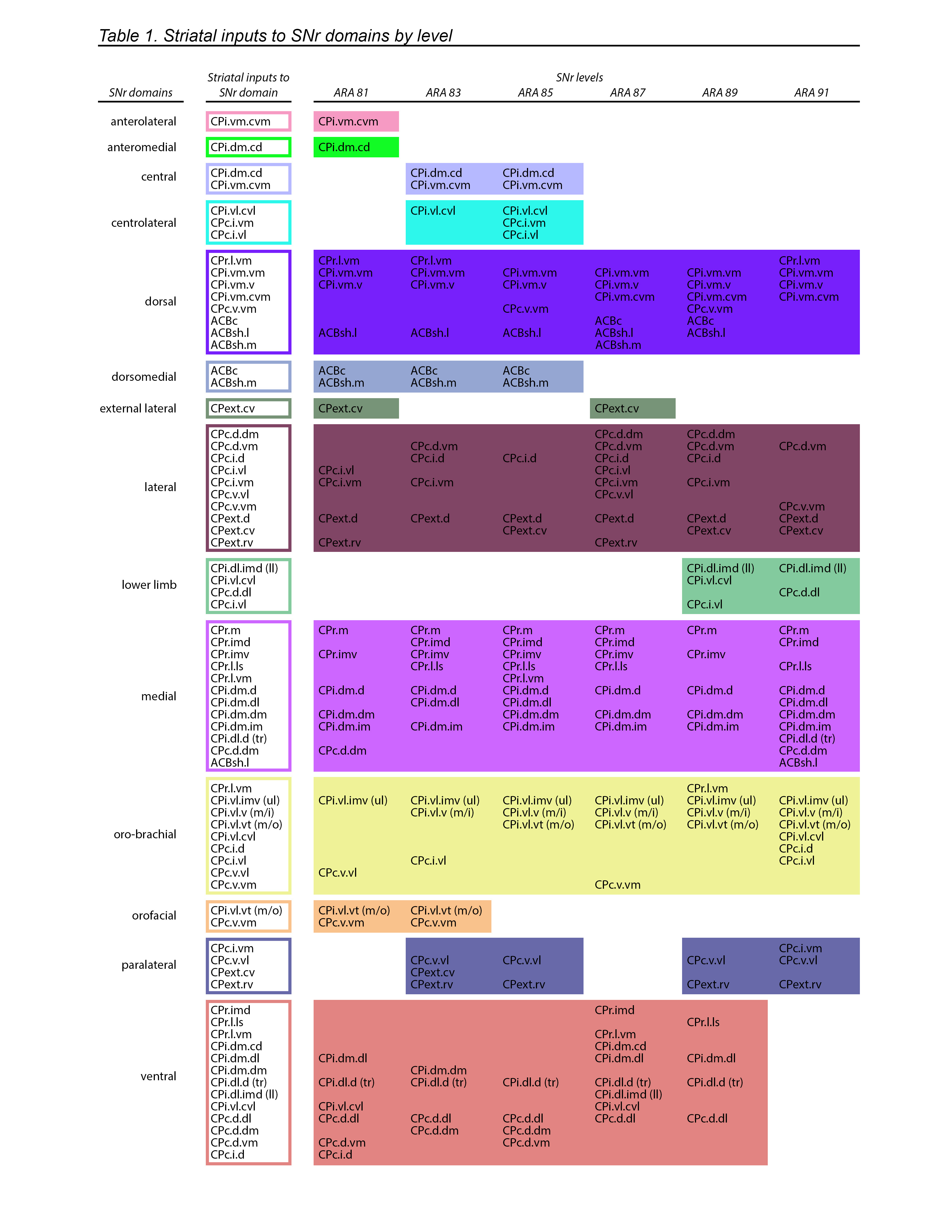
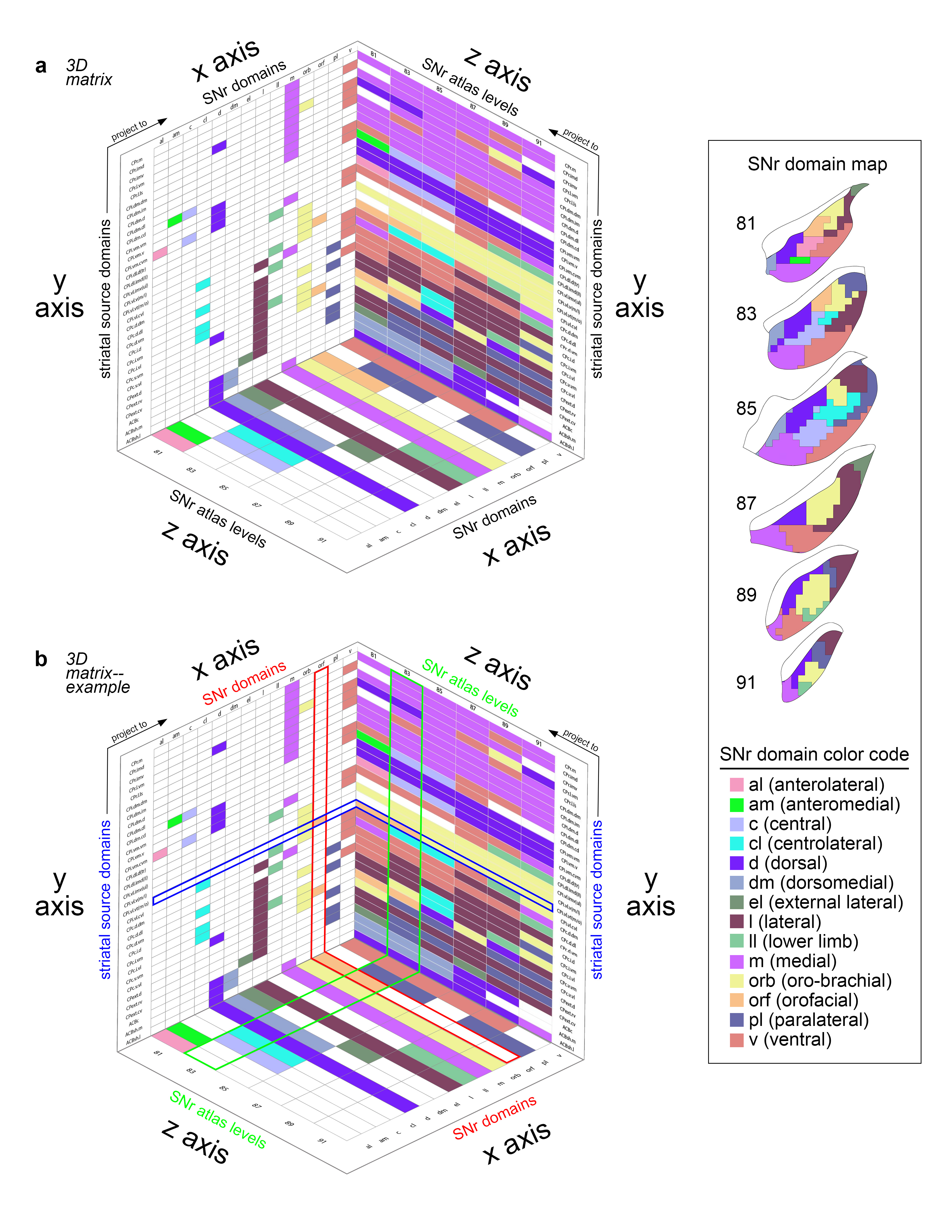
Extended Data Figure 7.jpg Extended Data Figure 7. 3D SNr matrix. a) The 3D matrix shows the relationships between the striatal source domains, the SNr domains, and the SNr atlas levels. The striatal source domains (on the y axis) send inputs to the domains of the SNr (x axis) across its atlas levels (i.e., rostrocaudal level in the ARA, z axis). The x-y plane identifies the striatal source domains and the SNr domains they contribute to, with color-codes indicating the SNr domain contributed to (see the SNr color code key and SNr domain map, right; white cells indicate no contribution). The y-z plane depicts the striatal source domains and to which level of the SNr they provide input, with color-codes indicating the SNr domain they contribute to at each representative atlas level. The x-z plane illustrates each SNr domain plotted according to the SNr atlas levels it is present at. b) As an example, the row for the outer mouth/facial striatal domain CPi.vl.vt (m/o) is highlighted blue. This domain contributes to two SNr domains, the oro-brachial and the orofacial, as indicated by the yellow and orange colored cells, respectively, in the blue highlighted row of the x-y plane. The column corresponding to the SNr orofacial domain is highlighted red, and it can be seen that this SNr domain has two striatal inputs, CPi.vl.vt (m/o) and CPc.v.vm. Following the blue highlighted row onto the y-z plane, it can be seen that the CPi.vl.vt (m/o) contributes to the SNr.orf at atlas levels 81 and 83 (orange cells) and it contributes to the SNr.orb at 85-91 (yellow cells). On the y-z plane, the column for atlas level 83 is highlighted green, and it can be seen that the other orange cell in that column corresponds to striatal input domain CPc.v.vm. On the x-z plane, the SNr orofacial domain is highlighted red, and it can be seen that this domain only spans two levels of the SNr, 81 and 83. This 3D graph illustrates all of the interrelated factors of the SNr domains, their striatal inputs, and the atlas levels at which each are present. |
 |
|
Extended Data Figure 8.jpg
|
 |
|
Extended Data Figure 9.jpg
|
 |
|
Extended Data Figure 10.jpg
|
 |
|
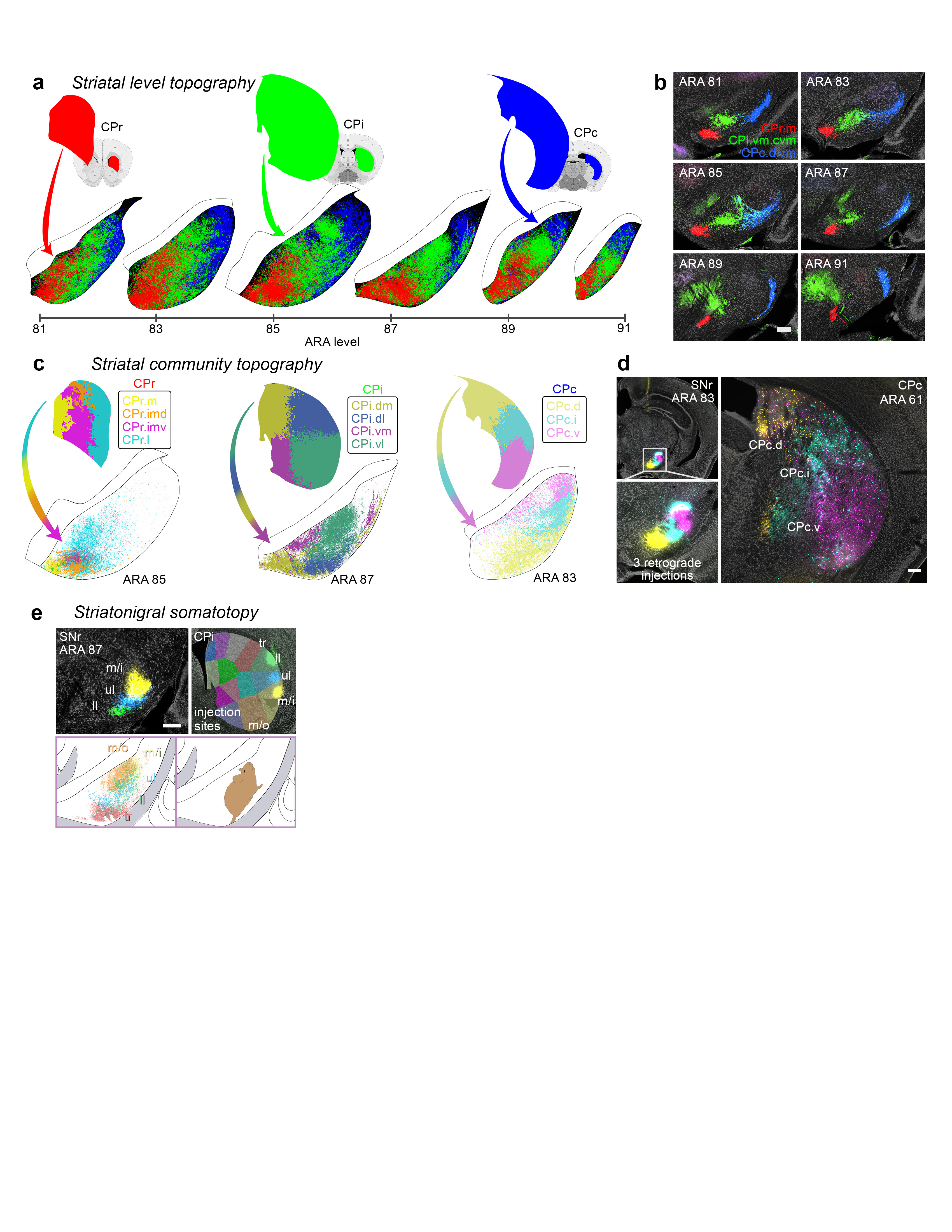
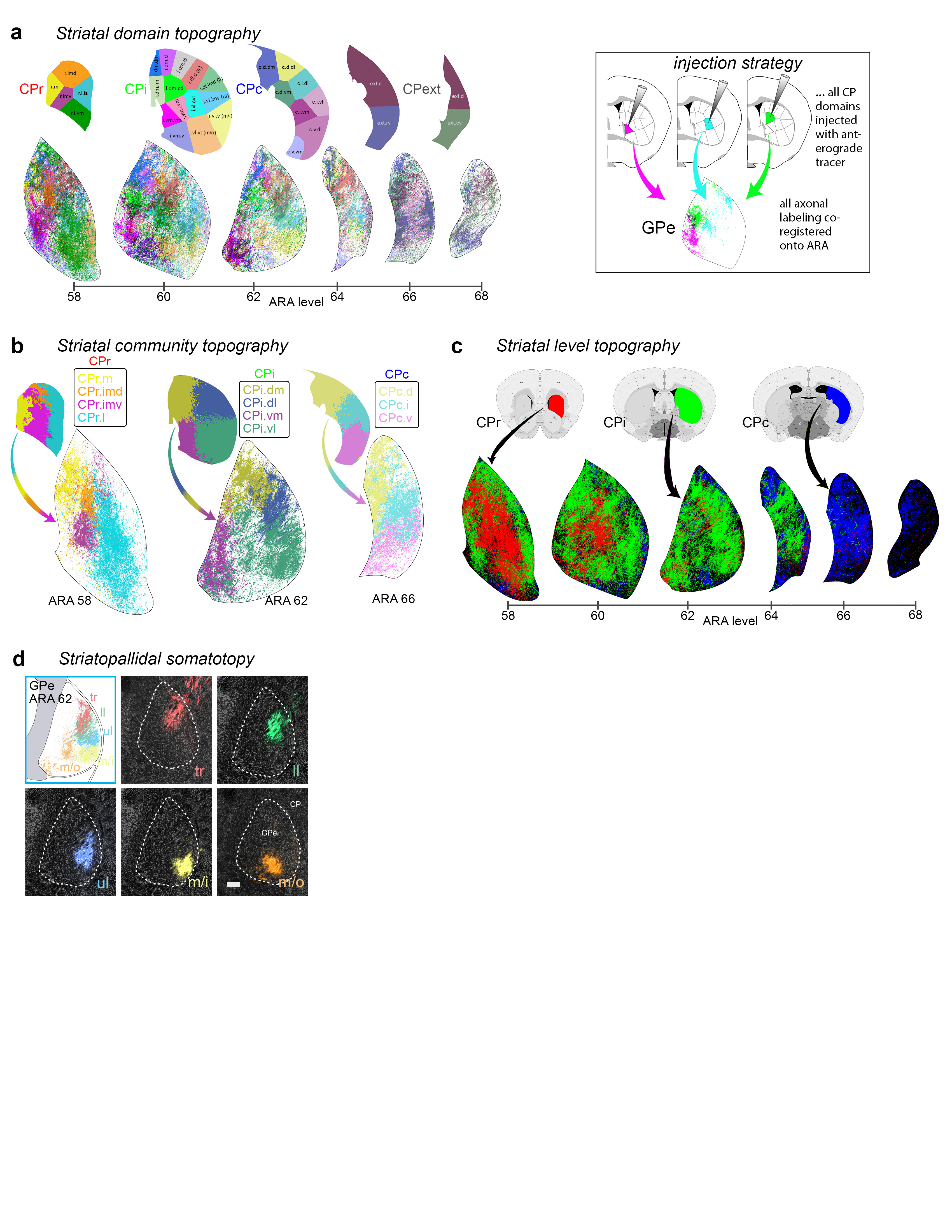
Extended Data Figure 11.jpg Extended Data Figure 11. GPe projection maps. The majority of striatal domains project to GPe with restricted terminal fields that have little overlap and convergence among one another. This largely parallelized striatopallidal topography is evident at the domain-, community-, and level-scale resolution in the reconstruction maps. a, Domain-level projection maps of all striatopallidal terminations, colored according to their striatal source domain. Collectively, the entire CP sends projections that cover the entire GPe. Projections from individual CP domains follow a rostral to rostral and caudal to caudal pattern (i.e., rostral CP to rostral GPe, etc.), a topography similar to the primate striatopallidal pathway (Hazrati & Parent, 1992). No projections from any individual CP domain span the entire rostrocaudal extent of the pallidum. b, Community-level view of striatopallidal terminations depicts axons of all CP domains colored to match their parent community (e.g., reconstructions of axons from CPi.dl.d and CPi.dl.imd are colored blue for community CPi.dl), revealing that the dorsoventral and mediolateral topography of the CP is generally maintained in the GPe. c, Axonal reconstructions originating from all striatal domains of rostral, intermediate, and caudal CP levels are colored red, green, or blue, respectively. The rostral-to-rostral and caudal-to-caudal striatopallidal topography is easily apparent in these maps. The CPext projects to the most caudal levels of GPe (not shown here). d, The somatotopic map in the GPe is revealed by striatopallidal terminations from body region-specific striatal source domains: trunk (tr), lower limb (ll), upper limb (ul), inner mouth (m/i), and outer mouth (m/o). The raw source images are shown in the photomicrographs (coronal plane, medial is left, scalebar = 200µm) and the axonal reconstructions in the co-registered connectivity map. Axons were pseudocolored to match their striatal source domain. |
 |
|
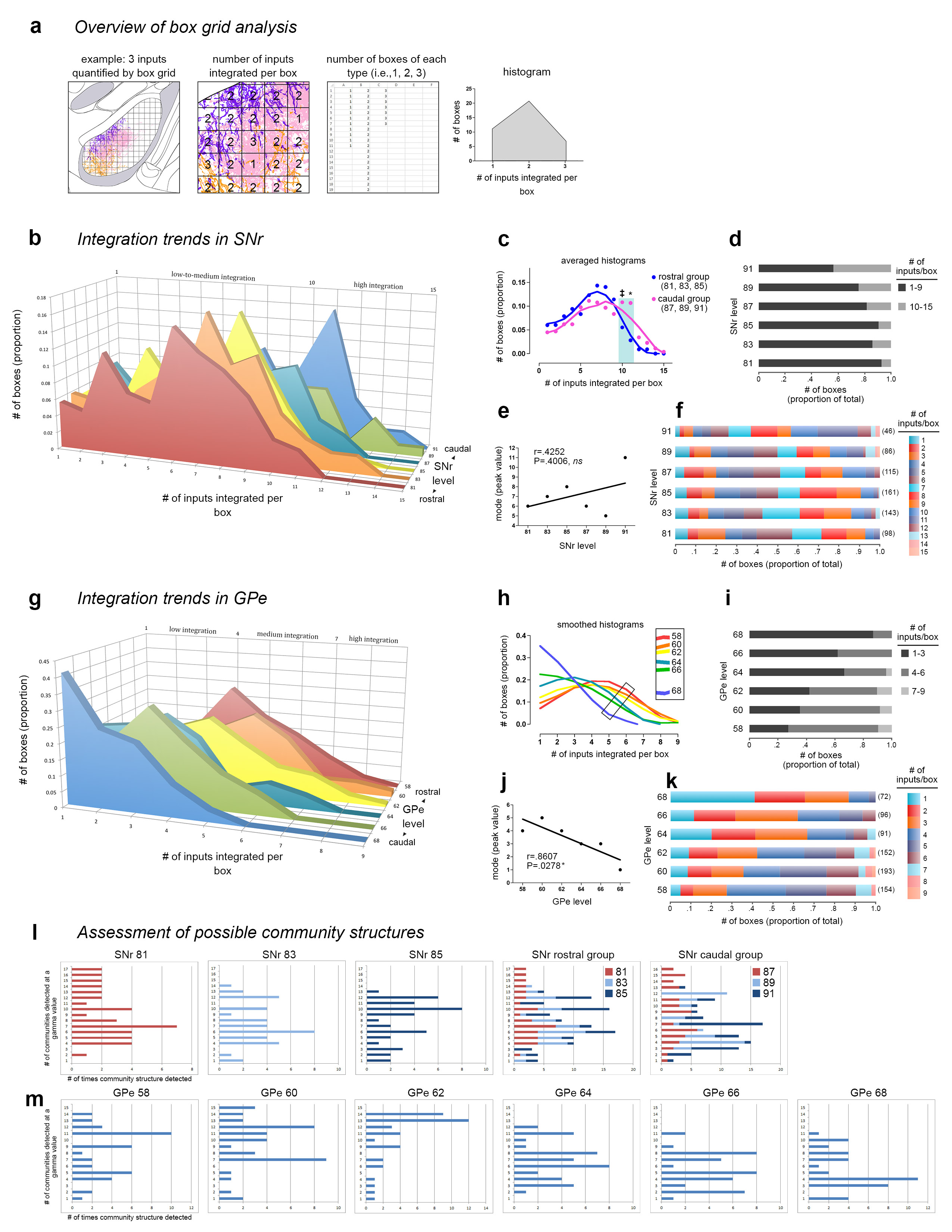
Extended Data Figure 12.jpg Extended Data Figure 12. Box grid quantification of striatal output data. Box grid data quantifies striatonigral and striatopallidal topography, describes integration trends in the pallidum and nigra, and serves as input data for the community analysis. The example in a, illustrates how the box grid analysis works using 3 inputs (pink, purple, and orange; left panel). Each whole and partial box in the ROI receives 1-3 inputs (center panel); the number of boxes of each input category is tallied (right panel) and plotted in a frequency distribution (histogram). b, Frequency distributions for each level of the SNr are shown rostral to caudal (front to back in the graph). The caudal 3 levels have a greater proportion of boxes devoted to integrating high numbers of inputs, as seen by the tails of their distributions sticking out in that range. This was validated statistically by comparing the caudal 3 and the rostral 3 distributions with ANOVA (* P<.0033, ‡ .05>P>.025), which are averaged and summarized in c. The proportion of boxes integrating various numbers of inputs at each level is represented in the stacked bar charts: d, shows a categorized graph, with low-to-moderate integration (1-9 inputs) in black and high integration (10-15 inputs) in gray; f, shows the same data with each bin in a different color (the bars from left to right correspond to the legend from top to bottom), and the numbers in parentheses at the end of each bar are the total number of boxes at each level. e, Regression analysis of the peak of each histogram from b with SNr level shows no correlation (r=0.4252, P=0.4006). g, Frequency distributions for each level of GPe are shown caudal to rostral (front to back in the graph). The distributions are fairly similar in shape and exhibit a linear trend, from rostral GPe integrating higher numbers of inputs per box and shifting to successively lower integration with each caudal level. Smoothing of the histograms and plotting them in a single plane in h highlights this stepwise trend from higher to lower integration, rostral to caudal, respectively (inset). j, This trend was found to be significant when assessed by regression analysis (r=0.8607, P=0.0278). Stacked bar graphs in i and k are as in d and f. l-m, The Louvain community detection algorithm was run multiple times over a range of gamma values, with gamma modulating the number of communities (i.e., domains) detected in the nigra or pallidum. The bar graphs show the different community structures detected (y axis) and how many times they were detected (x axis); each integral increment on the x axis means one gamma detected that community structure, so the peaks represent the most commonly detected community structures. These survey analyses were run for each nucleus-level, and results for SNr 81-85 can be seen individually and stacked together (SNr rostral group), along with the stacked graph for the SNr caudal group (SNr 87-91, individual graphs not shown). The individual graphs for GPe are shown in m. |
 |
|
Extended Data Figure 13.jpg Extended Data Figure 13. Direct and indirect pathway striatopallidal data. a, Direct and indirect pathway striatopallidal topography was compared by Cre-dependent tracing of D1 dopamine receptor-expressing (direct) and A2A adenosine receptor-expressing (indirect) medium spiny neurons. Injections of AAV-DIO-EGFP were made into the same region of dorsomedial (CPi.dm) or dorsolateral (CPi.dl) striatum in D1-Cre and A2A-Cre mouse lines (N=4, one for each target/Cre-line combination). Direct and indirect pathway terminals from the same striatal region had the same topography in the GPe. This property is also borne out at the single-cell resolution as seen in the fMOST data in b, where 2 indirect pathway neurons (red and orange) terminate in the same general region as 3 direct pathway neurons (blue, green, and aqua). Given that the direct pathway has “bridging collaterals” that terminate in the GPe (Cazorla et al. 2014), we demonstrate that both the direct and indirect pathways’ terminals in the GPe have the same topography when arising from the same striatal source region. Photomicrographs in a are coronal, medial is left, and scalebars = 200µm. |
 |
|
Extended Data Figure 14.jpg
|
 |
|
Extended Data Figure 15.jpg
|
 |
|
Extended Data Figure 16.jpg
|
 |
|
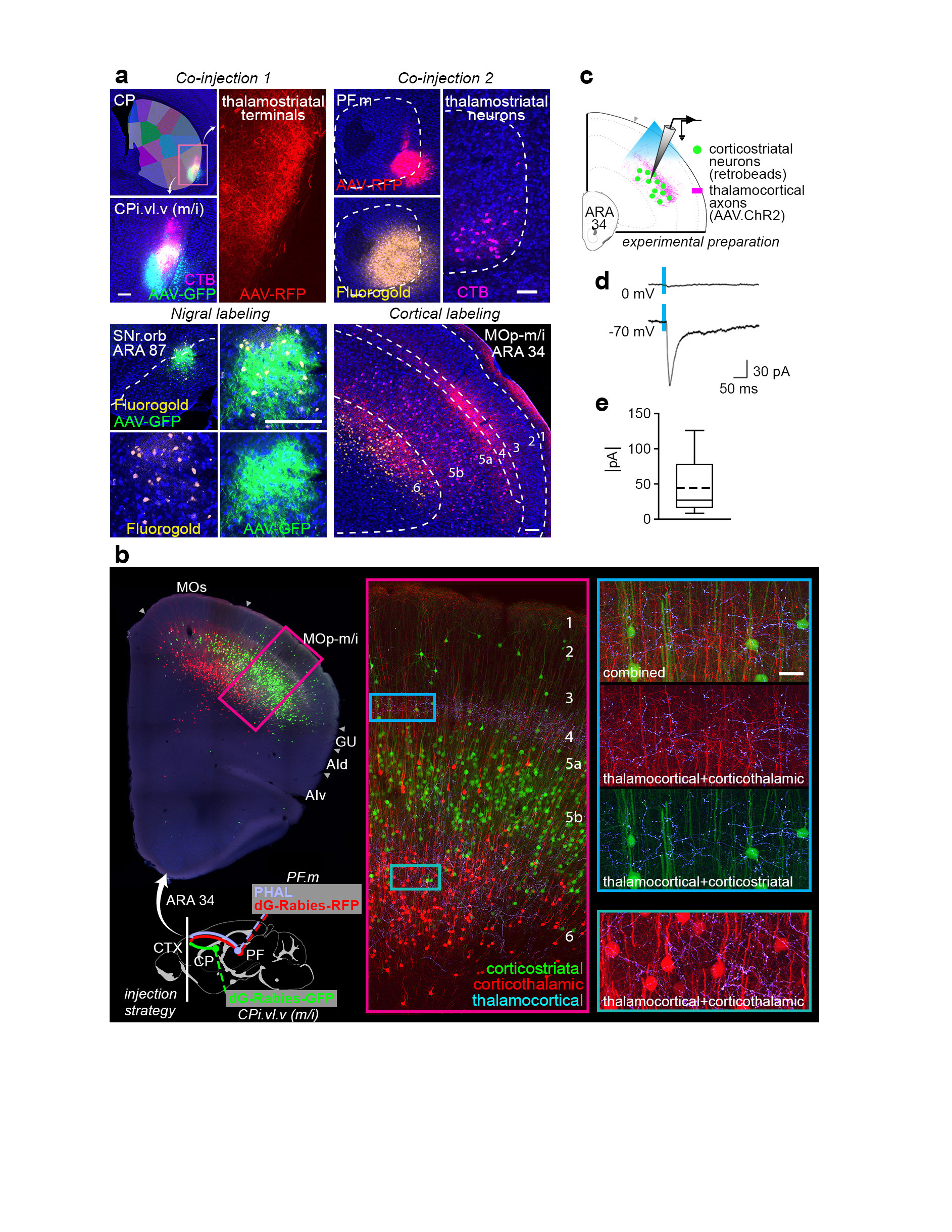
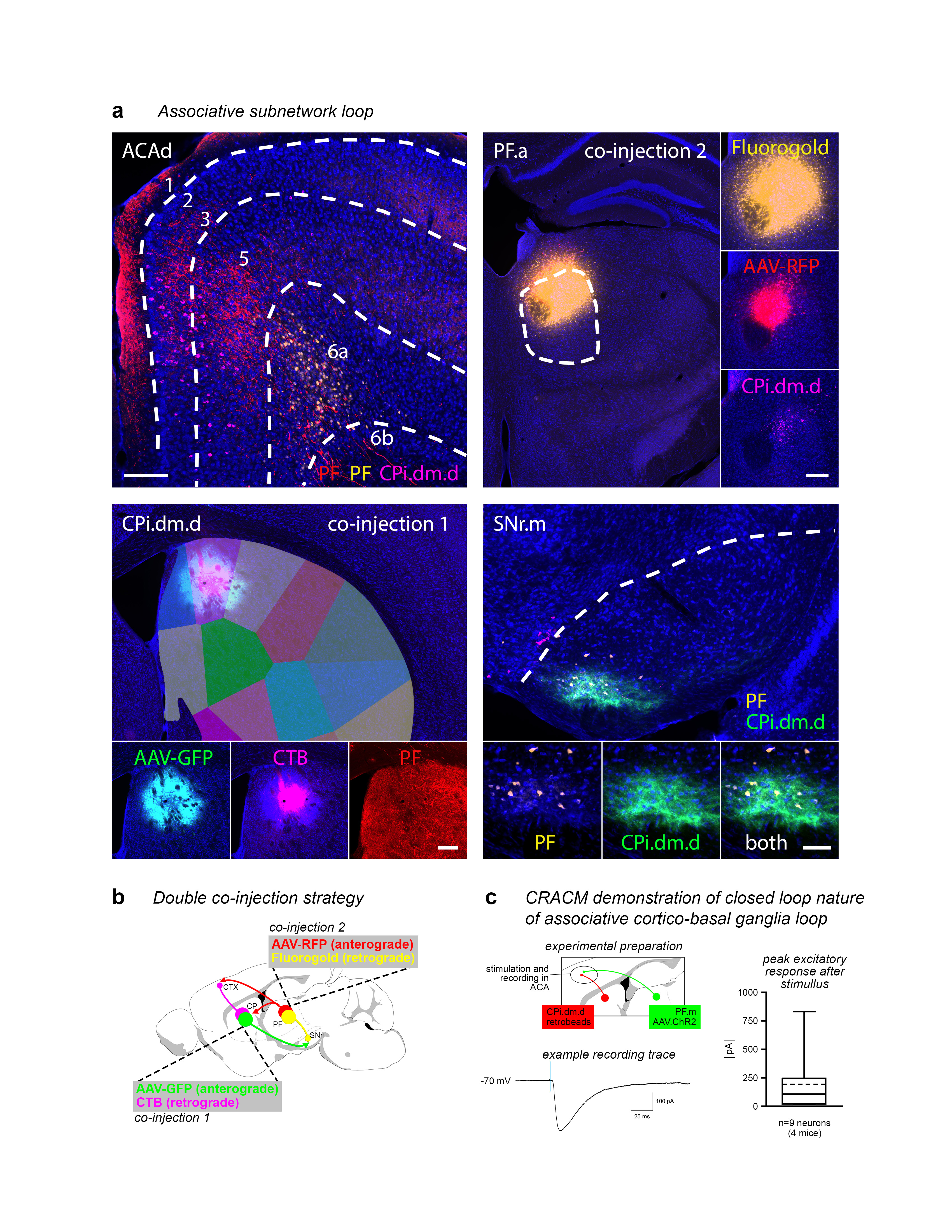
Extended Data Figure 17.jpg Extended Data Figure 17. Double co-injection demonstrating the associative subnetwork loop. a, One co-injection was placed in the striatum (CPi.dm.d, injected with AAV-GFP and CTB) and the other co-injection was made in the thalamus (PF.a, injected with AAV-RFP and Fluorogold). The transported tracers overlap in the cortex (ACAd) and nigra (SNr.m), revealing the discrete, closed-loop nature of the subnetwork (representative case from n=3). Note that the RFP-labeled axons in the striatum and CTB-labeled somata in the PF reveal the direct thalamostriatal pathway between those two nodes. b, The injection strategy and prototypical circuit are shown in schematic. c, The closed-loop nature of this loop was verified electrophysiologically. The CPi.dm.d was injected with retrobeads to retrogradely label corticostriatal neurons, and PF.m was injected with AAV.ChR2 rendering the thalamocortical axons optically excitable. Retrobead-labeled neurons in anterior cingulate cortex were patch clamped and recorded during blue light stimulation with tetrodotoxin and 4-aminopyridine in the bath solution to ensure monosynaptic responses only. Nine neurons were recorded from 4 mice, and all 9 showed responses to stimulation (meansd, 191.3±256.4 pA), confirming that the associative subnetwork loop has a substantial recurrent component. For box plot, box demarcates first and third quartiles, whiskers show min/max, solid line is median and dashed line is mean. All photomicrographs are coronal, medial is left, SNr scalebar 100 µm, all other scalebars 200 µm. |
 |
|
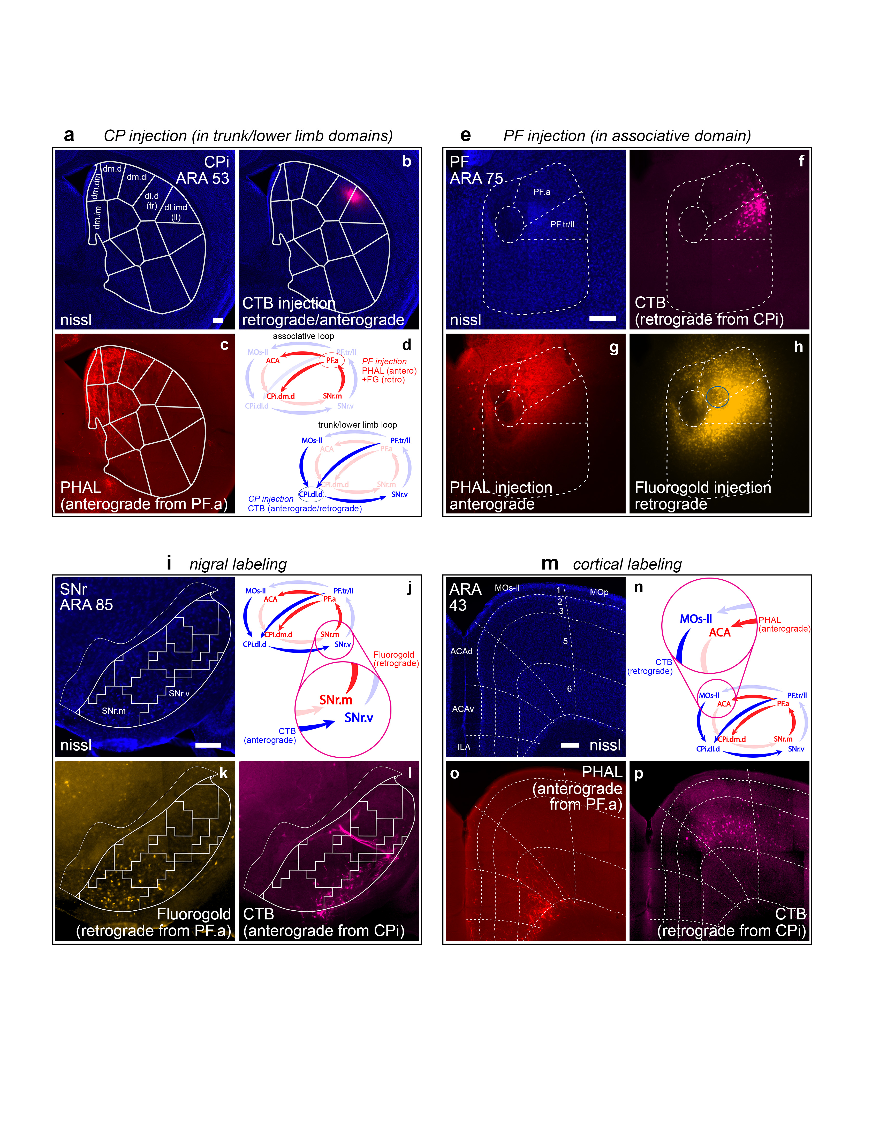
Extended Data Figure 18.jpg Extended Data Figure 18. Co-injections in separate, neighboring loops. To assess the degree of overlap between adjacent cortico-basal ganglia-thalamic loops, a double co-injection strategy was split across the a, trunk/lower limb and e, associative loops. b, An injection of CTB was made into the tr/ll domains of the CP. In this case, a high concentration of CTB (0.2%) was used, which results in both retrograde and anterograde labeling from the injection site. The retrograde labeling from this injection in the PF.tr/ll domain can be seen in f. e, In PF, a co-injection of g, PHAL and h, Fluorogold was made into the PF.a, adjacent to the PF.tr/ll. For clarity, the center of the FG injection site (the area of strongest uptake and transport of labeling) has been highlighted with a blue circle. The injection strategy and predicted labeling patterns are summarized in d. Dense anterograde labeling from the PHAL can be seen in c in the CP.dm.d and other domains of the CPi.dm but not in the tr/ll domains. The nigral and cortical labeling from the striatal and PF injections of these separate but neighboring loops shows only marginal overlap in their separate, adjacent regions in the i-j nigra and m-n cortex. The Fluorogold from PF.a strongly labels the k SNr.m while next to it the l SNr.v is labeled by anterograde CTB from the tr/ll domains of the CP. In the cortex, o, the PHAL labels the ACA while p, the retrograde CTB labels the adjacent MOs-ll. All photomicrographs are coronal, medial is left, and scalebars = 200µm. |
 |
|
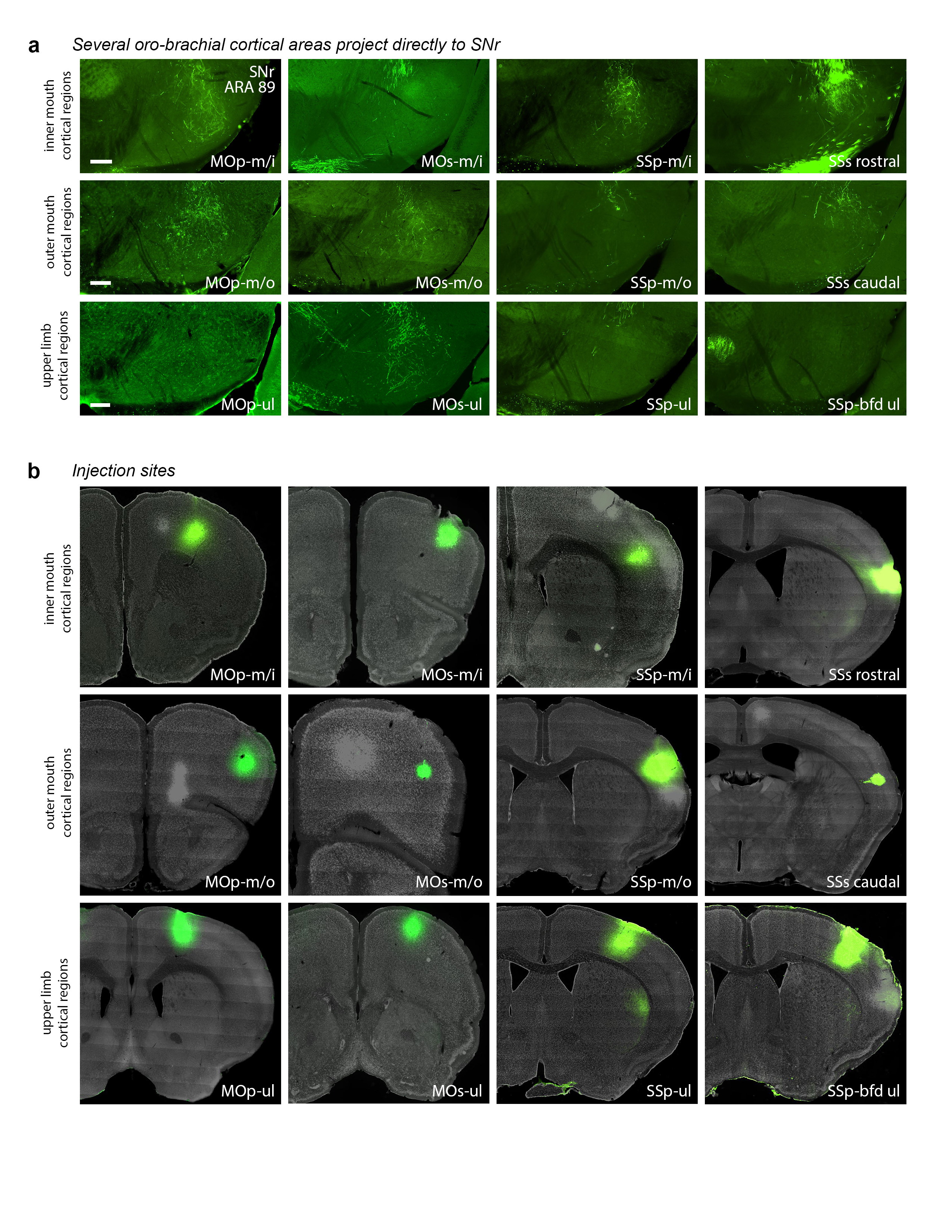
Extended Data Figure 19.jpg Extended Data Figure 19. Corticonigral data. a, Some but not all cortical regions of the inner mouth (m/i), outer mouth (m/o), and upper limb (ul) somatomotor subnetworks send direct axonal projections to the SNr.oro-brachial domain, as demonstrated by PHAL injections. b, Injection sites for the labeling in panel a. Other cortical regions do not appear to project directly to SNr (data not shown). All photomicrographs are coronal, medial is left, and scalebars = 200µm. |
 |
|
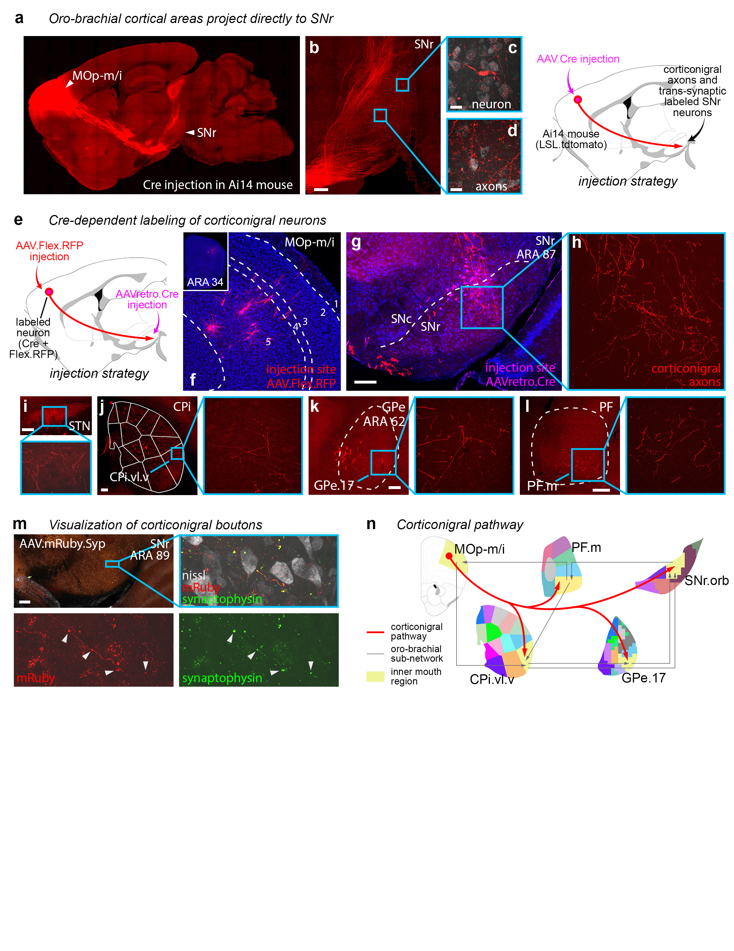
Extended Data Figure 20.jpg Extended Data Figure 20. The corticonigral pathway. a, The corticonigral pathway seen in sagittal section. Injection of AAV.Cre into inner mouth primary motor cortex (MOp-m/i) in Ai14 mouse (n=2) releases tdtomato expression in the corticofugal pathway, revealing axons in b, the SNr. In the insets, d, individual axons bearing terminal boutons are discernable, and c, an SNr neuron is labeled through anterograde transsynaptic infection of the AAV.Cre virus. e, The corticonigral pathway from MOp-m/i was validated using Cre-dependent labeling, by g, infecting cortical axons in the nigra with AAVretro.Cre, which f, unlocked fluorophore expression in MOp-m/i neurons injected with AAV.FLEX.RFP (n=2). h, The labeled MOp-m/i axons are seen in the SNr.orb, as well as the mouth domains of the j CP, k GPe, and l PF, as well as a restricted region of the i STN, indicating that at least some of these cortical neurons comprise the hyperdirect pathway. m, To visualize bona fide synaptic terminations in the SNr, the MOp-m/i was injected with AAV.mRuby.Syp-GFP (n=1), which labels axons with red fluorescence and synaptic boutons with green fluorescence (arrowheads). n, The corticonigral pathway appears to be a unique feature of the oro-brachial subnetwork, contacting all mouth regions in it and suggesting that cortex can simultaneously activate all other nodes in the subnetwork. Photomicrographs in f-m are coronal, medial is left. Scalebars in c-d = 20 µm, all others = 200 µm. |
 |